Draw a Circle at Intersection in Canvas
Basic graphics
Introduction
The path module allows one to construct PostScript-like paths, which are ane of the main building blocks for the generation of drawings. A PostScript path is an capricious shape consisting of straight lines, arc segments and cubic Bézier curves. Such a path does non have to be connected but may also incorporate several asunder segments, which volition be called subpaths in the following.
Todo
example for paths and subpaths (figure)
Usually, a path is constructed by passing a list of the path primitives moveto , lineto , curveto , etc., to the constructor of the path class. The following code snippet, for case, defines a path p that consists of a straight line from the point \((0, 0)\) to the point \((1, 1)\)
from pyx import * p = path . path ( path . moveto ( 0 , 0 ), path . lineto ( i , 1 )) Equivalently, one can besides use the predefined path subclass line and write
p = path . line ( 0 , 0 , 1 , 1 ) While already some geometrical operations can be performed with this path (see side by side section), another PyX object is needed in order to actually existence able to draw the path, namely an instance of the sail course. By convention, we employ the proper name c for this case:
In club to draw the path on the sail, nosotros use the stroke() method of the sheet class, i.eastward.,
c . stroke ( p ) c . writeEPSfile ( "line" ) To complete the case, we have added a writeEPSfile() call, which writes the contents of the canvas to the file line.eps . Note that an extension .eps is added automatically, if non already present in the given filename. Similarly, if you want to generate a PDF or SVG file instead, utilize
or
c.writeSVGfile("line")
As a second example, allow us ascertain a path which consists of more than one subpath:
cross = path . path ( path . moveto ( 0 , 0 ), path . rlineto ( 1 , ane ), path . moveto ( 1 , 0 ), path . rlineto ( - ane , 1 )) The get-go subpath is over again a straight line from \((0, 0)\) to \((1, 1)\), with the but departure that we now have used the rlineto course, whose arguments count relative from the last point in the path. The second moveto example opens a new subpath starting at the point \((one, 0)\) and ending at \((0, 1)\). Note that although both lines intersect at the point \((ane/2, i/2)\), they count as disconnected subpaths. The full general rule is that each occurrence of a moveto instance opens a new subpath. This ways that if i wants to describe a rectangle, one should non use
rect1 = path . path ( path . moveto ( 0 , 0 ), path . lineto ( 0 , one ), path . moveto ( 0 , 1 ), path . lineto ( ane , 1 ), path . moveto ( 1 , 1 ), path . lineto ( 1 , 0 ), path . moveto ( ane , 0 ), path . lineto ( 0 , 0 )) which would construct a rectangle out of four asunder subpaths (see Fig. Rectangle case a). In a better solution (see Fig. Rectangle case b), the pen is non lifted between the first and the terminal point:
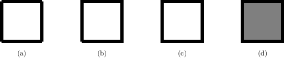
Rectangle example
Rectangle consisting of (a) four separate lines, (b) i open path, and (c) i closed path. (d) Filling a path always closes it automatically.
rect2 = path . path ( path . moveto ( 0 , 0 ), path . lineto ( 0 , i ), path . lineto ( 1 , one ), path . lineto ( 1 , 0 ), path . lineto ( 0 , 0 )) However, equally one tin encounter in the lower left corner of Fig. Rectangle example b, the rectangle is withal incomplete. It needs to be closed, which can exist done explicitly past using for the concluding straight line of the rectangle (from the point \((0, 1)\) back to the origin at \((0, 0)\)) the closepath directive:
rect3 = path . path ( path . moveto ( 0 , 0 ), path . lineto ( 0 , 1 ), path . lineto ( one , 1 ), path . lineto ( 1 , 0 ), path . closepath ()) The closepath directive adds a straight line from the electric current indicate to the offset betoken of the current subpath and furthermore closes the sub path, i.e., it joins the offset and the cease of the line segment. This results in the intended rectangle shown in Fig. Rectangle example c. Notation that filling the path implicitly closes every open subpath, as is shown for a single subpath in Fig. Rectangle example d), which results from
c . stroke ( rect2 , [ deco . filled ([ colour . gray ( 0.5 )])]) Hither, nosotros supply as second argument of the stroke() method a listing which in the present example only consists of a single element, namely the then called decorator deco.filled . Equally its proper name says, this decorator specifies that the path is not merely being stroked but also filled with the given color. More information about decorators, styles and other attributes which tin be passed equally elements of the list can be institute in Sect. Attributes: Styles and Decorations. More details on the available path elements can be found in Sect. Path elements.
To conclude this section, we should not forget to mention that rectangles are, of course, predefined in PyX, so above we could have every bit well written
rect2 = path . rect ( 0 , 0 , 1 , 1 ) Hither, the first two arguments specify the origin of the rectangle while the second two arguments define its width and height, respectively. For more details on the predefined paths, we refer the reader to Sect. Predefined paths.
Path operations
Oft, one wants to perform geometrical operations with a path earlier placing information technology on a canvas by stroking or filling it. For example, i might desire to intersect ane path with some other one, divide the paths at the intersection points, and and then join the segments together in a new style. PyX supports such tasks past ways of a number of path methods, which we will introduce in the following.
Suppose you want to draw the radii to the intersection points of a circle with a straight line. This task can be done using the post-obit lawmaking which results in Fig. Example: Intersection of circumvolve with line yielding two radii
from pyx import * c = sail . sheet () circle = path . circle ( 0 , 0 , 2 ) line = path . line ( - iii , 1 , three , 2 ) c . stroke ( circumvolve , [ style . linewidth . Thick ]) c . stroke ( line , [ fashion . linewidth . Thick ]) isects_circle , isects_line = circumvolve . intersect ( line ) for isect in isects_circle : isectx , isecty = circumvolve . at ( isect ) c . stroke ( path . line ( 0 , 0 , isectx , isecty )) c . writePDFfile () 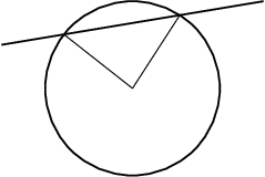
Example: Intersection of circle with line yielding two radii
Here, the basic elements, a circumvolve around the indicate \((0, 0)\) with radius \(2\) and a straight line, are divers. Then, passing the line, to the intersect() method of circumvolve, nosotros obtain a tuple of parameter values of the intersection points. The starting time element of the tuple is a list of parameter values for the path whose intersect() method has been chosen, the 2nd element is the corresponding listing for the path passed equally argument to this method. In the nowadays case, we only need one list of parameter values, namely isects_circle. Using the at() path method to obtain the point respective to the parameter value, we depict the radii for the dissimilar intersection points.
Another powerful feature of PyX is its ability to split paths at a given set of parameters. For case, in guild to make full in the previous example the segment of the circle delimited by the direct line (cf. Fig. Case: Intersection of circle with line yielding radii and circumvolve segment), one first has to construct a path corresponding to the outline of this segment. The post-obit code snippet yields this segment
arc1 , arc2 = circle . split ( isects_circle ) if arc1 . arclen () < arc2 . arclen (): arc = arc1 else : arc = arc2 isects_line . sort () line1 , line2 , line3 = line . split up ( isects_line ) segment = line2 << arc 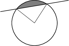
Instance: Intersection of circle with line yielding radii and circle segment
Here, we first split the circle using the carve up() method passing the list of parameters obtained above. Since the circle is airtight, this yields two arc segments. We so use the arclen() , which returns the arc length of the path, to discover the shorter of the 2 arcs. Before splitting the line, we have to accept into business relationship that the split up() method only accepts a sorted listing of parameters. Finally, we join the straight line and the arc segment. For this, we brand employ of the << operator, which non but adds the paths (which could be washed using line2 + arc ), merely likewise joins the concluding subpath of line2 and the first one of arc. Thus, segment consists of just a single subpath and filling works as expected.
An important issue when operating on paths is the parametrisation used. Internally, PyX uses a parametrisation which uses an interval of length \(i\) for each path element of a path. For instance, for a simple direct line, the possible parameter values range from \(0\) to \(1\), respective to the start and concluding signal, respectively, of the line. Appending another straight line, would extend this range to a maximal value of \(2\).
However, the situation becomes more complicated if more circuitous objects similar a circle are involved. Then, ane could be tempted to assume that over again the parameter value ranges from \(0\) to \(1\), because the predefined circle consists just of 1 arc together with a closepath element. Still, this is not the example: the actual range is much larger. The reason for this behaviour lies in the internal path handling of PyX: Earlier performing any non-trivial geometrical operation on a path, it will automatically be converted into an example of the normpath class (see too Sect. path.normpath ). These and so generated paths are already separated in their subpaths and only comprise straight lines and Bézier curve segments. XXX explain normpathparams and things like p.begin(), p.stop()-1,
A more geometrical manner of accessing a point on the path is to use the arc length of the path segment from the first indicate of the path to the given point. Thus, all PyX path methods that accept a parameter value also allow the user to pass an arc length. For case,
from math import pi r = 2 pt1 = path . circle ( 0 , 0 , r ) . at ( r * pi ) pt2 = path . circle ( 0 , 0 , r ) . at ( r * three * pi / 2 ) c . stroke ( path . path ( path . moveto ( * pt1 ), path . lineto ( * pt2 ))) will draw a straight line from a point at bending \(180\) degrees (in radians \(\pi\)) to some other point at bending \(270\) degrees (in radians \(3\pi/two\)) on a circle with radius \(r=2\). Note however, that the mapping from an arc length to a point is in general discontinuous at the beginning and the end of a subpath, and thus PyX does not guarantee whatever particular effect for this boundary case.
More information on the bachelor path methods tin be plant in Sect. Course path — PostScript-similar paths.
Attributes: Styles and Decorations
Attributes ascertain properties of a given object when it is beingness used. Typically, at that place are different kinds of attributes which are unremarkably orthogonal to each other, while for one type of attribute, several choices are possible. An instance is the stroking of a path. At that place, linewidth and linestyle are different kind of attributes. The linewidth might be thin, normal, thick, etc., and the linestyle might exist solid, dashed etc.
Attributes ever occur in lists passed as an optional keyword statement to a method or a function. Usually, attributes are the commencement keyword argument, and then i can just pass the list without specifying the keyword. Once more, for the path case, a typical telephone call looks similar
c . stroke ( path , [ style . linewidth . Thick , style . linestyle . dashed ]) Here, nosotros too encounter another characteristic of PyX'southward attribute arrangement. For many attributes useful default values are stored equally fellow member variables of the bodily attribute. For instance, style.linewidth.Thick is equivalent to fashion.linewidth(0.04, type="w", unit="cm") , that is \(0.04\) width cm (see Sect. Module unit for more information about PyX's unit arrangement).
Another important characteristic of PyX attributes is what is call attributed merging. A trivial example is the following:
# the following 2 lines are equivalent c . stroke ( path , [ style . linewidth . Thick , way . linewidth . sparse ]) c . stroke ( path , [ style . linewidth . thin ]) Here, the style.linewidth.thin aspect overrides the preceding style.linewidth.Thick declaration. This is specially important in more circuitous cases where PyX defines default attributes for a sure operation. When calling the respective methods with an attribute listing, this list is appended to the list of defaults. This fashion, the user can hands override certain defaults, while leaving the other default values intact. In addition, every aspect kind defines a special articulate attribute, which allows to selectively delete a default value. For path stroking this looks like
# the following two lines are equivalent c . stroke ( path , [ manner . linewidth . Thick , fashion . linewidth . articulate ]) c . stroke ( path ) The clear attribute is too provided by the base classes of the various styles. For instance, style.strokestyle.clear clears all strokestyle subclasses i.east. style.linewidth and style.linestyle . Since all attributes derive from attr.attr , you tin can remove all defaults using attr.clear . An overview over the most important attribute types provided past PyX is given in the following tabular array.
| Aspect category | description | examples |
|---|---|---|
| | decorator specifying the way the path is drawn | |
| | style used for path stroking | |
| | manner used for path filling | |
| | type of path filling | |
| | operations changing the shape of the path | |
| | attributes used for typesetting | |
| | transformations applied when drawing object | |
Todo
specify which classes in the table are in fact instances
Note that operations commonly allow for sure attribute categories just. For example when stroking a path, text attributes are not immune, while stroke attributes and decorators are. Some attributes might belong to several attribute categories similar colours, which are both, stroke and fill attributes.
Last, we discuss another important feature of PyX's attribute organisation. In order to allow the easy customisation of predefined attributes, it is possible to create a modified aspect by calling of an attribute instance, thereby specifying new parameters. A typical example is to modify the mode a path is stroked or filled by constructing advisable deco.stroked or deco.filled instances. For instance, the code
c . stroke ( path , [ deco . filled ([ color . rgb . light-green ])]) draws a path filled in green with a black outline. Here, deco.filled is already an case which is modified to fill with the given color. Note that an equivalent version would be
c . draw ( path , [ deco . stroked , deco . filled ([ colour . rgb . green ])]) In particular, you tin can come across that deco.stroked is already an attribute instance, since otherwise you were not allowed to pass it as a parameter to the draw method. Another case where the modification of a decorator is useful are arrows. For example, the following code draws an arrow head with a more acute bending (compared to the default value of \(45\) degrees):
c . stroke ( path , [ deco . earrow ( angle = 30 )]) Todo
changeable attributes
Source: https://pyx-project.org/manual/graphics.html
0 Response to "Draw a Circle at Intersection in Canvas"
Post a Comment